Statistics
$\def\F{\mathscr{F}} \def\R{\mathbb{R}} \def\E{\mathbb{E}} \def\N{\mathbb{N}} \def\mc{\mathcal} \def\Im{\text{Im}} \def\Var{\text{Var}} \def\MSE{\text{MSE}} \def\abs#1{|#1|} \def\bigabs#1{\left|#1\right|} \def\st{~|~} \def\set#1{\{#1\}} \def\condset#1#2{\{#1~|~#2\}} \def\bf{\mathbf} \def\bb{\mathbb}$
Descriptive statistics (measures of location and spread, order statistics, statistics of association, related figures). Discrete and continuous random variables (RV). Random sampling. Parametric probabilistic models (distributions) of RV. Central limit theorem. Likelihood principle, point and interval estimates. Statistical inference – hypotheses testing, significance level, confidence coefficient. Testing of hypotheses in one sample, two samples, more than two samples (including one sample, two sample and paired t-tests, ANOVA and post-hoc tests), goodness-of-fit tests. Linear regression model. (MV013)
Other Sources
Descriptive Statistics
Statistical Data Types
- nominal (sex, region, type of faults, …)
- no ordering of the values; just qualitative names
- ordinal (education, opinion, …)
- qualitative names with an ordering
- interval (temperature with the Celsius cale, year, …)
- values serve for comparisons, but do not correspond to any absolute value
- ratio (mass, length, duration, …)
- if the scale and the position of zero are fixed
Measures of Location
We are looking for a typical value. Assume the data is sorted so $x_1$ is the lowest value and $x_n$ the largest.
Mean: $\bar{x} = \frac{1}{n}{\sum_{i = 1}^n{x_i}}$
Median: $\tilde{x} = x_{\frac{n+1}{2}}$ for $n$ odd, $\tilde{x} = \frac{1}{2} (x_{\frac{n}{2}} + x_{\frac{n}{2}+1})$ for $n$ even
Mode: The value that appears most often in a set of data values.
$\alpha$-trimmed mean: Arithmetic mean after removing bottom and top $\alpha \in [0, 0.5)$ of the sorted values.
$\alpha$-winsorized mean: Arithmetic mean after replacing bottom and top $\alpha \in [0, 0.5)$ of the sorted values with the lower/upper bound of the not-replaced values.
$\alpha$-quantile: $q_\alpha = x_{\lceil n\alpha \rceil}$
- splits data into two parts: $\lceil n\alpha \rceil$ observations less or equal than the value, the rest greater or equal
- $0.5$-quantile = median, $0.25$-quantile is the first quartile ($Q_1$), $0.75$-quantile is the third quartile ($Q_3$)
- there are more definitions of quantile that can be used (at least 9)
For categorical variables, we can use:
- Ordinal data: median (quantiles), mode
- Nominal data: mode
Measures of Variability
We are looking for dispersion, scatter, or spread of the data.
Variance: $s^2 = \frac{1}{n - 1} \sum_{i = 1}^n (x_i - \bar{x})^2$
Standard deviation: $s = \sqrt{s^2}$
Range: $R = x_n - x_1$
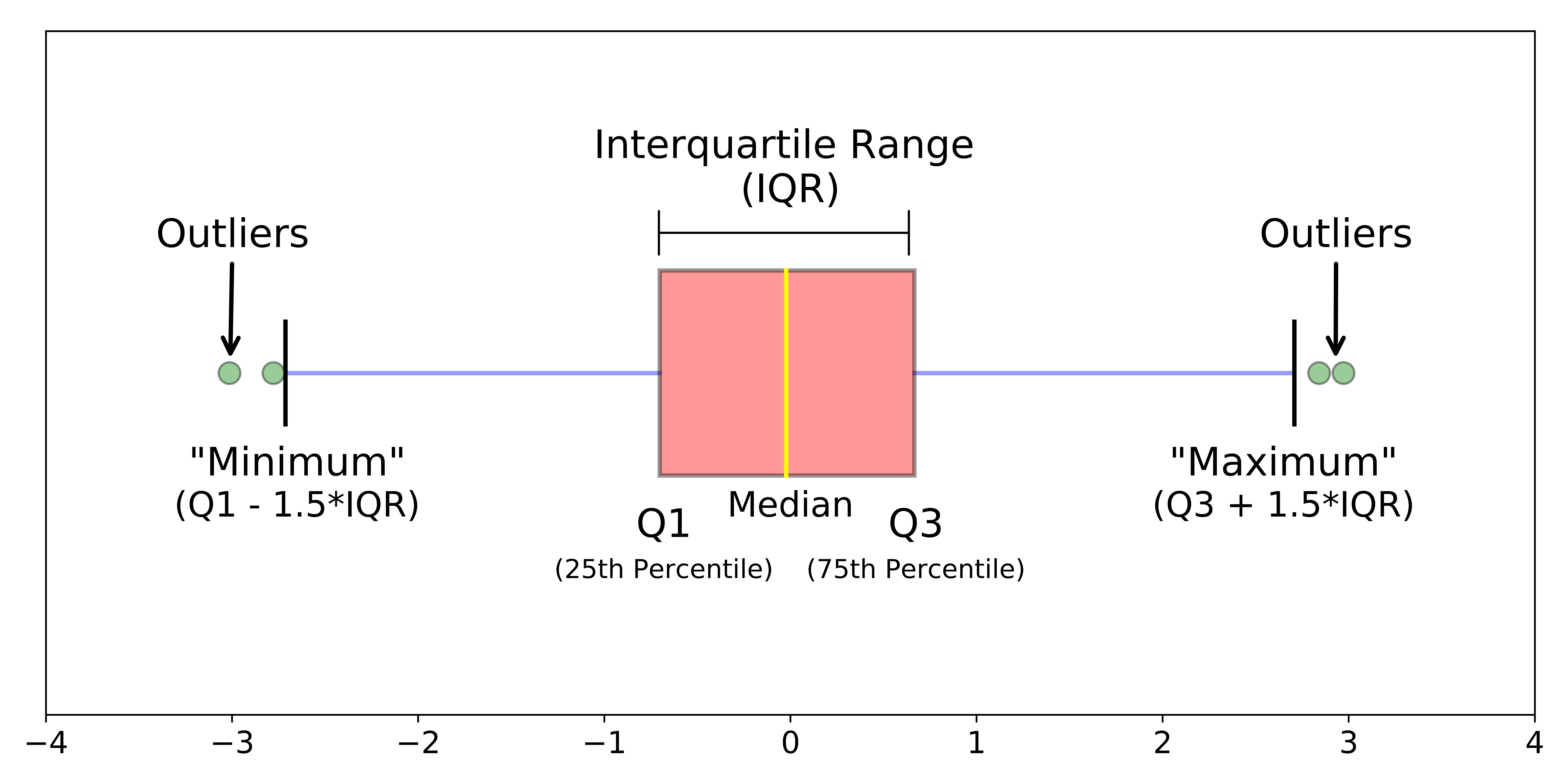
Interquartile range: $\text{IQR} = Q_3 - Q_1$
Median absolute deviation: $\text{MAD} = \text{median} \set{\abs{x_1 - \tilde{x}}, \dots, \abs{x_n - \tilde{x}}}$
For categorical variables, we compute heterogeneity:
- Denote $p_i = \frac{n_i}{n}$ the relative frequency of $i$-th category, where $n_i$ is the number of observations from $i$-th category for $i = 1, \dots, k$
- Zero heterogeneity: $p_i = 1$ for some $i$
- Maximal heterogeneity: $p_i = \frac{1}{k}$ for all $i$
- Gini index: $G = 1 - \sum_{i = 1}^k p_i^2$, $G \in [0, 1 - \frac{1}{k}]$
- Entropy: $E = -\sum_{i = 1}^k p_i \log{p_i}$, $E \in [0, \log{k}]$
Order Statistics
The $i$-th order statistic of the sample is the $i$-th lowest value of the sample ($x_i$).
Statistics of Association
Denote $\bf{x} = (x_1, \dots, x_n)^T$ and $\bf{y} = (y_1, \dots, y_n)^T$.
(Sample) Covariance: $c = \frac{1}{n - 1} \sum_{i=1}^n (x_i - \bar{x}) (y_i - \bar{y})$
(Sample) Pearson Correlation: $r = \frac{c}{s_x s_y} = \frac{\sum_{i=1}^n (x_i - \bar{x})(y_i - \bar{y})}{\sqrt{\sum_{i=1}^n(x_i - \bar{x})^2 \sum_{i = 1}^n (y_i - \bar{y})^2}}$
Related Figures
Boxplot
Histogram
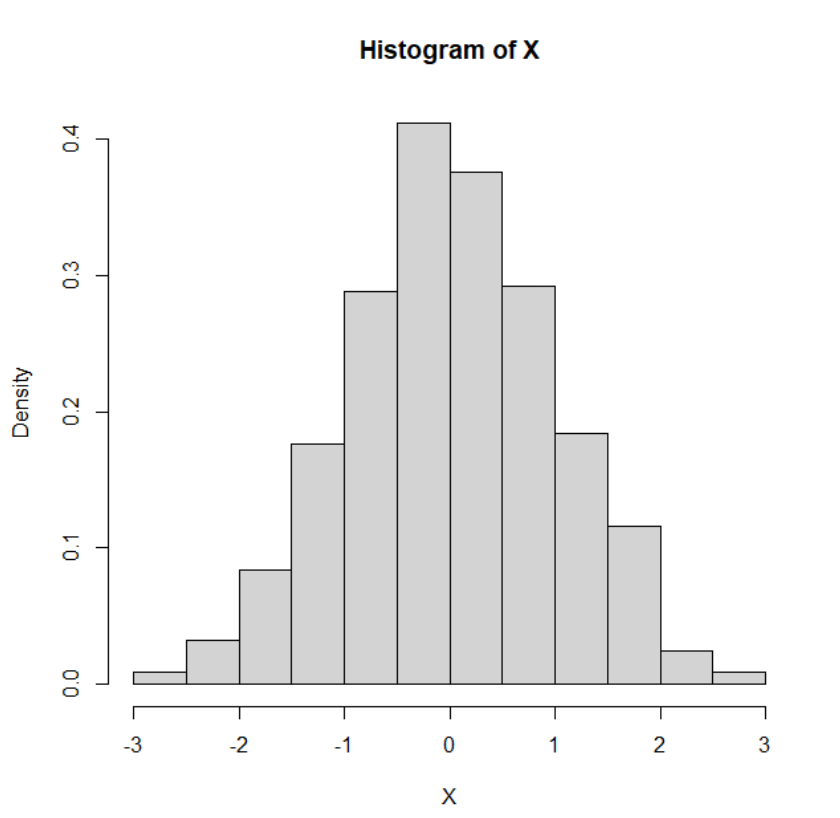
It is a piecewise constant estimate of the distribution of the data. The first step is to bin the range of values into a series of $k$ equal-sized intervals.
Categorical Variables
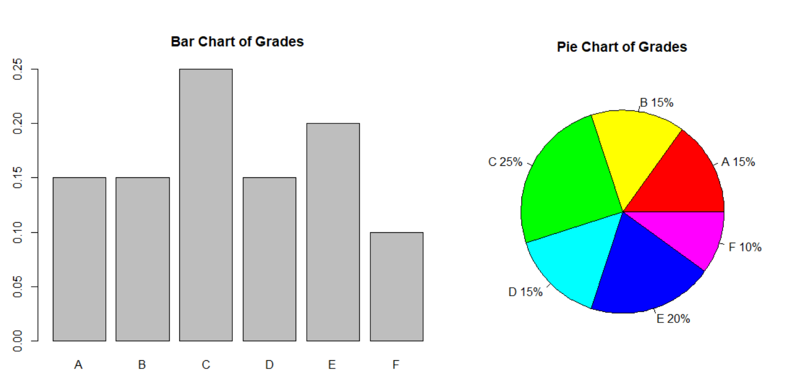
- pie chart, bar chart
- graphs of frequencies or relative frequencies
Scatter Plot
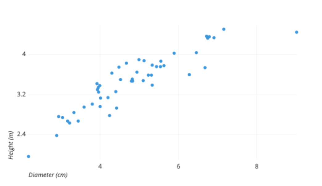
Is a plot that displays values for two variables of the dataset using Cartesian coordinates (measure of correlation).
Discrete and Continuous Random Variables
The probability framework is described in Probability, Theory of Information.
Let $(\Omega, \mc{A}, P)$ be a probability space. The measurable mapping $X: \Omega \to \R$ is called a random variable.
Random variable $X$ is discrete, if there exists a finite or countable set $\set{x_1, x_2, \dots}$ such that $P(X = x_i) > 0$ and $\sum_{i = 1}^\infty P(X = x_i) = 1$.
Random variable $X$ is (absolutely) continuous, if there exists an integrable and nonnegative function $f = f_X$ such that $F(x) = \int_{-\infty}^x f(t) dt$ for all $x \in \R$.
Random Sampling
Data represent results of some measurement (experiment) or a sample from a population (survey). We consider a representative random sample from a population, as compiling data about the entire population (census) is expensive and time-consuming.
Representative sampling assures that inferences and conclusions can be extended from the sample to the population as a whole.
Parametric Probabilistic Models (distributions) of RV
Discrete Univariate Distributions
Bernoulli Distribution
A random variable $X$ has Bernoulli distribution with $p \in (0, 1)$ if the pmf of $X$ is given by
\[p(x) = P(X = x) = \left\{ \begin{array}{ll} 1 - p, & x = 0, \\ p, & x = 1, \\ 0, & \text{otherwise.} \end{array}\right.\]$X$ describes events with two outcomes (success, failure) with $p$ the probability of success.
$\E X = p, \Var(X) = p(1 - p)$
Binomial Distribution
$n \in \N, p \in (0, 1)$
\[p(x) = P(X = x) = \left\{ \begin{array}{ll} \binom{n}{x} p^x (1 - p)^{n - x}, & x=0, 1, \dots, n,\\ 0, & \text{otherwise.} \end{array}\right.\]$X$ represents the number of successes in $n$ repeated independent Bernoulli trials with $p$ the probability of success at each individual trial.
$\E X = np, \Var(X) = np(1 - p)$
Poisson Distribution
$\lambda > 0$
\[p(x) = P(X = x) = \left\{ \begin{array}{ll} \frac{\lambda^k e^{-\lambda}}{k!}, & x=0, 1, \dots,\\ 0, & \text{otherwise.} \end{array}\right.\]$X$ represents the number of events occuring in a fixed interval of time if these events occur independently of the time since the last event. $\lambda$ is equal to the expected number of events in the specified interval.
Poisson distribution is a special case of the binomial distribution, where (in the limit) $n \to \infty$ and $p \to 0$.
$\E X = \lambda, \Var(X) = \lambda$
Geometric Distribution
$p \in (0, 1)$
\[p(x) = P(X = x) = \left\{ \begin{array}{ll} p(1 - p)^x, & x=0, 1, \dots,\\ 0, & \text{otherwise.} \end{array}\right.\]$X$ represents the number of failures before the first success when repeating the independent Bernoulli trials with $p$ the probability of success at each individual trial.
Geometric distribution is the only discrete memoryless probability distribution.
$\E X = \frac{1 - p}{p} = \frac{1}{p} - 1, \Var(X) = \frac{1 - p}{p^2}$
Discrete Uniform Distribution
$A \subset \R$
\[p(x) = P(X = x) = \left\{ \begin{array}{ll} \frac{1}{\abs{A}}, & x \in A,\\ 0, & \text{otherwise.} \end{array}\right.\]All the values of $X$ are equally probable.
Continuous Univariate Distributions
Continuous Uniform Distribution
A random variable $X$ has continuous uniform distribution on the interval $(a, b) \subset \R$, if the pdf of $X$ is given by
\[f(x) = \left\{ \begin{array}{ll} \frac{1}{b - a}, & x \in (a, b),\\ 0, & \text{otherwise.} \end{array}\right.\]All the values of $X$ are equally probable (but probability of $X$ being $x \in (a, b)$ is $0$ for all $x$).
$\E X = \frac{a+b}{2}, \Var(X) = \frac{(b - a)^2}{12}$
Exponential Distribution
$\lambda > 0$
\[f(x) = \left\{ \begin{array}{ll} \lambda e^{-\lambda x}, & x \geq 0,\\ 0, & \text{otherwise.} \end{array}\right.\]Random variable $X$ represents time between two events in a Poisson point process.
Exponential distribution is the only continuous memoryless distribution.
$\E X = \frac{1}{\lambda}, \Var(X) = \frac{1}{\lambda^2}$
Standard Normal Distribution
\[f(x) = \frac{1}{\sqrt{2\pi}}e^{-\frac{x^2}{2}}, x \in \R.\]$\E X = 0, \Var(X) = 1$
The cdf of $x$ cannot be expressed by a closed formula and must be tabulated.
Normal Distribution
$\mu \in \R, \sigma^2 > 0$
\[f(x) = \frac{1}{\sqrt{2\pi \sigma^2}}e^{-\frac{(x - \mu)^2}{2 \sigma^2}}, x \in \R.\]$\E X = \mu, \Var(X) = \sigma^2$
$\frac{X - \mu}{\sigma}$ has a standard normal distribution.
Other Distributions
- Cauchy distribution: for $A, B \sim \mc{N}(0, 1)$, $X = \frac{A}{B}$ has Cauchy distribution $\text{Cauchy}(0, 1)$.
- expected value and variance are undefined
- $\chi^2$ with $n \in \N$ degrees of freedom: sum of $n$ squared independent random variables $Z_i$ with $Z_i \sim \mc{N}(0, 1)$
- Student’s t-distribution: $X = \frac{Z}{\sqrt{V / n}}$ has t-distribution with $n$ degrees of freedom if $Z \sim \mc{N}(0, 1), V \sim \chi^2(n)$
- Fisher-Snedecor F-distribution: $X = \frac{U / n_1}{V / n_2}$ for $U \sim \chi^2(n_1), V \sim \chi^2(n_2)$ has F-distribution with $n_1$ and $n_2$ degrees of freedom
Central Limit Theorem
Lindeberg-Lévy CLT
Let $X_1, \dots, X_n$ be i.i.d. random variables with $\E X_i = \mu$ and $\Var(X_i) = \sigma^2 > 0$. Then the random variable
\[\frac{\bar{X} - \mu}{\sigma / \sqrt{n}}\]has asymptotically standard normal distribution $\mc{N}(0, 1)$ as $n \to \infty$.
It follows that for $n$ large enough, $S = \sum_{i=1}^n X_i \approx \ \mc{N}(n\mu, n\sigma^2)$ and $\bar{X} \approx \mc{N}(\mu, \frac{\sigma^2}{n})$.
Moivre-Laplace CLT
Let $X_n$ be a random variable with the $\text{Binomial}(n, p)$ distribution. Then random variable
\[\frac{X_n - np}{\sqrt{np(1-p)}}\]has asymptotically as $n \to \infty$ standard normal distribution $\mc{N}(0, 1)$.
It follows that $X_n \approx \mc{N}(np, np(1 - p))$ for $n$ large enough. It is recommended that $np \geq 5$ and $n(1 - p) \geq 5$.
Parameter Estimates
Point Estimates
Parametric model: Let $\bb{X} = (X_1, \dots, X_n)^T$ be a random sample with cdf $F(x, \bb{\theta})$, where $\bb{\theta} \in \bb{\Theta} \subset \R^p$ is an unknown parameter and $F$ is a known function.
Point estimate: Let $\bb{X} = (X_1, \dots, X_n)^T$ be a random sample with cdf $F(x, \theta)$. A function $T$ of $X_1, \dots, X_n$ is a point estimate of $\theta$.
- $T$ is unbiased estimate of $\theta$ if $\E T = \theta$ for all $\theta \in \Theta$.
- $T$ is asymptotically unbiased estimate of $\theta$ if $\lim_{n \to \infty}{\E T} = \theta$ for all $\theta \in \Theta$.
- $T$ is (weak) consistent estimate of $\theta$ if for all $\varepsilon > 0$, $\lim_{n \to \infty} P(\abs{T - \theta} > \varepsilon) = 0$, for all $\theta \in \Theta$.
Let $T$ be an estimator of parameter $\theta$. Then the mean squared error of $T$ is defined as
\[\MSE(T) = \E(T - \theta)^2\]
If $T$ is an unbiased estimate of $\theta$, then $\MSE(T) = \Var(T)$. Mean squared error depends on the unknown value $\theta$.
The estimate that minimizes the mean squared error for all $\theta$ uniformly does not exist.
Let $\bf{X} = (X_1, \dots, X_n)^T$ be a random sample from a distribution with mean $\mu$ and variance $\sigma^2$. Then
- The sample mean $\bar{X} = \frac{1}{n} \sum_{i=1}^n X_i$ is unbiased and consistent estimate of $\mu$.
- The sample variance $S^2 = \frac{1}{n-1} \sum_{i=1}^n (X_i - \bar{X})^2$ is unbiased and consistent estimate of $\sigma^2$.
Likelihood Principle
The likelihood principle states that in making inference or decisions about the state of the nature all the relevant experimental information is given by the likelihood function.
(this was not mentioned in MV013)
Maximum Likelihood Method
Let $\bf{X} = (X_1, \dots, X_n)^T$ be a random sample with cdf $F(x, \bf{\theta})$. Assume that there exists a pmf (for discrete variables) or pdf (for continuous variables) of $X_i$. Denote it $f(x, \bf{\theta})$.
- Denote $L(\bf{\theta}) = \prod_{i = 1}^n f(x_i, \bf{\theta})$ the joint pdf (pmf) of the random sample $\bf{X}$.
- $L(\bf{\theta})$ as a function of $\bf{\theta}$ is called the likelihood function (for fixed $x_1, \dots, x_n$).
- Maximum likelihood estimate of $\bf{\theta}$ is then $\hat{\bf{\theta}} = \arg\max_\bf{\theta} L(\bf{\theta})$.
- Function $l(\bf{\theta}) = \log L(\bf{\theta}) = \sum_{i = 1}^n \log f(x_i, \bf{\theta})$ is called the log-likelihood function.
- Maximum likelihood estimate is also the argmax of the log-likelihood.
Under mild conditions (regularity), the MLE $\hat{\bf{\theta}}$:
- is asymptotically unbiased estimate of $\bf{\theta}$.
- is consistent estimate of $\bf{\theta}$.
- has asymptotically $p$-dimensional normal distribution.
- MLE of a parametric function $\gamma(\bf{\theta})$ is $\gamma(\hat{\bf{\theta}})$.
Method of Moments
Assume that $\E X_i^p < \infty$.
- Denote $\mu^\prime_1 = \mu^\prime_1(\bf{\theta}) = \E X_i^1, \dots, \mu^\prime_p = \E X_i^p$ the moments of $X_i$.
- Denote $M_k = \frac{1}{n} \sum_{i=1}^n X_i^k$ for $k = 1, 2, \dots, p$ the sample moments.
If $\E X_i^p < \infty$, then $M_k$ is unbiased and consistent estimate of $\mu^\prime_k$ for all $k = 1, \dots, p$.
Interval Estimates
Assume that $X_1, \dots, X_n$ is a random sample with cdf $F(x, \theta)$. Interval $[L, U] = [L(X_1, \dots, X_n), U(X_1, \dots, X_n)]$ is $(1 - \alpha) \cdot 100\%$ confidence interval for parameter $\theta$, if
$P(L \leq \theta \leq U) = 1 - \alpha$, for all $\theta \in \Theta$.
- $L$ and $U$ are random variables.
- The number $1 - \alpha$ is called the confidence level (confidence coefficient). Typically $\alpha = 0.05$.
One-sided CI:
Interval $[L, \infty)$ is $(1 - \alpha) \cdot 100\%$ lower (left) confidence interval for parameter $\theta$, if
$P(L \leq \theta) = 1 - \alpha$, for all $\theta \in \Theta$.
Interval $(-\infty, U]$ is $(1 - \alpha) \cdot 100\%$ upper (right) confidence interval for parameter $\theta$, if
$P(\theta \leq U) = 1 - \alpha$, for all $\theta \in \Theta$.
Construction of Confidence Intervals
- We find a pivotal statistic - a function $h$ of a random sample $X_1, \dots, X_n$ and the parameter $\theta$. The pivotal statistic’s distribution does not depend on $\theta$, therefore $h$ is a random variable.
-
We find $\alpha/2$ and $1 - \frac{\alpha}{2}$ quantiles of the distribution of the pivotal statistic $h(X_1, \dots, X_n, \theta)$, i.e.
\[P(q_{\alpha/2} \leq h(X_1, \dots, X_n, \theta) \leq q_{1 - \frac{\alpha}{2}}) = 1 - \alpha\] -
We adjust the values in the inequalities to transform $h$ into $\theta$
\[P(L \leq \theta \leq U) = 1 - \alpha\] - The interval $[L, U]$ is then the $(1 - \alpha) \cdot 100\%$ confidence interval for $\theta$.
- Factors affecting the width of the confidence interval: sample size, confidence level, variability of the data
Model Assumptions
- $X_1, \dots, X_n$ is a random sample - i.i.d.
- $X_i$ is normally distributed
- if not, we use the same test statistic, because the sample mean with a large number of samples still follows the normal distribution by CLT
- we need a sufficient number of observations for the approximation to be accurate ($n \geq 30$)
- the underlying variance $\sigma^2$ must be finite in that case
Statistical Inference
Statistical inference makes propositions about a population, using data drawn from the population with some form of sampling.
The conclusion of a statistical inference is a statistical proposition. Some common forms of statistical proposition are:
- a point estimate
- an interval estimate (confidence interval)
- rejection of a hypothesis
- clustering/classification of data points into groups
Hypotheses Testing
Assume that $X_1, \dots, X_n$ is a random sample with cdf $F(x, \bf{\theta})$, where $\bf{\theta} \in \bf{\Theta}$ is an unknown parameter. Our goal is to decided between two competing hypotheses about parameters $\bf{\theta}$:
- $H_0: \bf{\theta} \in \bf{\Theta_0}$ - the null hypothesis
- $H_1: \bf{\theta} \in \bf{\Theta_1}$ - the alternative hypothesis
- $\bf{\Theta_0} \cap \bf{\Theta_1} = \emptyset, \bf{\Theta_0} \cup \bf{\Theta_1} = \bf{\Theta}$
We can either:
- reject the null hypothesis $H_0$ (The null hypothesis is not true, therefore the alternative is.)
- not reject the null hypothesis $H_0$ (The null hypothesis might be true, or we do not have enough information to disprove.)
- WE CANNOT SAY WE ACCEPT THE NULL HYPOTHESIS!
| decision/reality | $H_0$ is true | $H_1$ is true |
|---|---|---|
| We reject $H_0$ | type I error | ✓ |
| We do not reject $H_0$ | ✓ | type II error |
We want to minimize probabilities of both types of error, but we cannot control both at the same time. Type I error is more serious than type II error.
Therefore, we choose $\alpha > 0$ (significance level) so that $P(\text{type I error}) = \alpha$. Typically $\alpha = 0.05$. Then we search for a suitable statistical test with probability of type II error as small as possible.
The test is given by a test statistic and a critical region.
- Test statistic $T$ is a function of the random sample.
- Critical region $W$ is a set of values of the test statistic $T$ for which we reject $H_0$.
Construction of the test statistic and the critical region:
- First, we have to find a pivotal statistic for a given model.
- Test statistic $T$ it the value of the pivotal statistic under $H_0$.
- We need to know what the distribution of the test statistic is under the null hypothesis.
-
We define the critical region $W$ so that $P(\text{type I error}) = \alpha$.
- If $T \in W$, then we reject $H_0$.
- If $T \not\in W$, then we do not reject $H_0$.
We will consider these types of hypotheses:
- $H_0: \theta = \theta_0$, where $\theta_0$ is known.
- $H_1: \theta \not= \theta_0$ (two-sided alternative)
- $H_1: \theta > \theta_0$ (one-sided right alternative)
- $H_1: \theta < \theta_0$ (one-sided left alternative)
$p$-value
$p$-value is the probability under $H_0$ of obtaining test result at least as extreme as the result actually observed.
- If $p$-value is smaller than $\alpha$, we reject $H_0$.
- If $p$-value is greater than $\alpha$, we do not reject $H_0$.
Denote $t$ the observed value of test statistic $T$ for our data. $p$-value is then given by
- $2 \min\set{P(T \geq t \st H_0), P(T \leq t \st H_0)}$ for two-sided alternative
- $P(T \geq t \st H_0)$ for one-sided right alternative.
- $P(T \leq t \st H_0)$ for one-sided left alternative.
We use $(1 - \alpha) \cdot 100\%$ confidence intervals for $\theta$ for hypotheses testing. If $\theta_0$ belongs to the CI, we do not reject $H_0$.
Testing of Hypotheses
One-Sample $t$-Test
The one-sample $t$-test is a statistical hypothesis test used to determine whether an unknown population mean is different from a specific value.
Under $H_0$, the test statistic $T \sim t(n - 1)$.
- Model: $X_1, \dots, X_n$ is a random sample from a normal distribution $\mc{N}(\mu, \sigma^2)$.
- Null hypothesis: $H_0: \mu = \mu_0$.
- Test statistic: $T = \sqrt{n}\frac{\bar{X} - \mu_0}{S}$. Its value is denoted by $t$.
- Both-sided alternative: $H_1: \mu \not= \mu_0$
- $W = (-\infty, -t_{1 - \alpha/2}(n - 1)) \cup (t_{1 - \alpha/2}(n - 1), \infty)$
- $p$-value is $2 \min\set{F_T(t, n - 1), 1 - F_T(t, n - 1)}$
- CI for $\mu$: $[\bar{X} - t_{1 - \alpha/2}(n - 1) \frac{S}{\sqrt{n}}, \bar{X} + t_{1 - \alpha/2}(n - 1) \frac{S}{\sqrt{n}}]$
- Left-sided alternative: $H_1: \mu < \mu_0$
- CI for $\mu$: $(-\infty, \bar{X} + t_{1 - \alpha}(n - 1)\frac{S}{\sqrt{n}}]$
- Right-sided alternative: $H_1: \mu > \mu_0$
- CI for $\mu$: $[\bar{X} - t_{1 - \alpha}(n - 1)\frac{S}{\sqrt{n}}, \infty)$
If the data do not come from a normal distribution, we should not use one sample $t$-test, but the Z test instead (if the sample size is large enough to invoke CLT).
Z Test
Under $H_0$, the test statistic $Z \approx \mc{N(0, 1)}$.
- Model: $X_1, \dots, X_n$ is a random sample from a normal distribution $\mc{N}(\mu, \sigma^2)$.
- Null hypothesis: $H_0: \mu = \mu_0$.
- Test statistic: $Z = \sqrt{n}\frac{\bar{X} - \mu_0}{S}$. Its value is denoted by $z$.
- Both-sided alternative: $H_1: \mu \not= \mu_0$
- $W = (-\infty, -z_{1 - \alpha/2}(n - 1)) \cup (z_{1 - \alpha/2}(n - 1), \infty)$
- approximate $p$-value is $2 \min\set{\theta(z), 1 - \theta(z)}$ where $\theta$ is the cdf of $\mc{N}(0, 1)$,
- CI for $\mu$: $[\bar{X} - z_{1 - \alpha/2}(n - 1) \frac{S}{\sqrt{n}}, \bar{X} + z_{1 - \alpha/2}(n - 1) \frac{S}{\sqrt{n}}]$
- Left-sided alternative: $H_1: \mu < \mu_0$
- CI for $\mu$: $(-\infty, \bar{X} + z_{1 - \alpha}(n - 1)\frac{S}{\sqrt{n}}]$
- Right-sided alternative: $H_1: \mu > \mu_0$
- CI for $\mu$: $[\bar{X} - z_{1 - \alpha}(n - 1)\frac{S}{\sqrt{n}}, \infty)$
Normality Testing
Some statistical test require the normality of data (for example, the $t$ test). We have a few methods for checking the normality of the data:
- histogram + plot of pdf with estimated parameters
- kernel density + plot of pdf with estimated parameters
- plot of empirical cdf
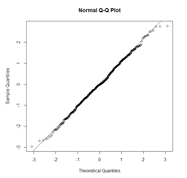
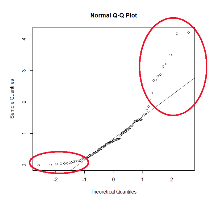
- Q-Q plot
- P-P plot
Q-Q Plot
Compares empirical and theoretical quantiles on two axes.
P-P Plot
Compares empirical and theoretical distribution functions.
Statistical Testing for Normality
- $H_0$: $F$ is cdf of normal distribution with $\mu$ and $\sigma$ parameters
-
$H_1$: $F$ is not cdf of a normal distribution
- tests based on skewness and kurtosis
- Jarque-Bera test
- Shapiro-Wilk test
- Kolmogorov-Smirnov test - measures distance between empirical cdf and the theoretical cdf
- $\chi^2$ goodness of fit test
Pearson’s $\chi^2$ Goodness-of-fit Test
The goodness of fit of a statistical model describes how well it fits a set of observations. Measures of goodness of fit typically summarize the discrepancy between observed values and the values expected under the model in question.
We use the test to check whether the data we obtained could possibly come from a distribution of our choice.
The Pearson’s chi-squared test statistic is defined by $\theta^2 = \sum_{i}\frac{(O_i - N p_i)^2}{N p_i}$, where $O_i$ is the count of samples from the $i$-th bin/category, $\sum_i O_i = N$, and $p_i$ is the probability of the $i$-th bin according to our chosen distribution.
The test statistic has the $\chi^2$ distribution with $df = \text{Cats} - \text{Params}$ degrees of freedom, where $\text{Cats}$ is the number of categories recognized by the model and $\text{Parms}$ number of fitted parameters in the distribution.
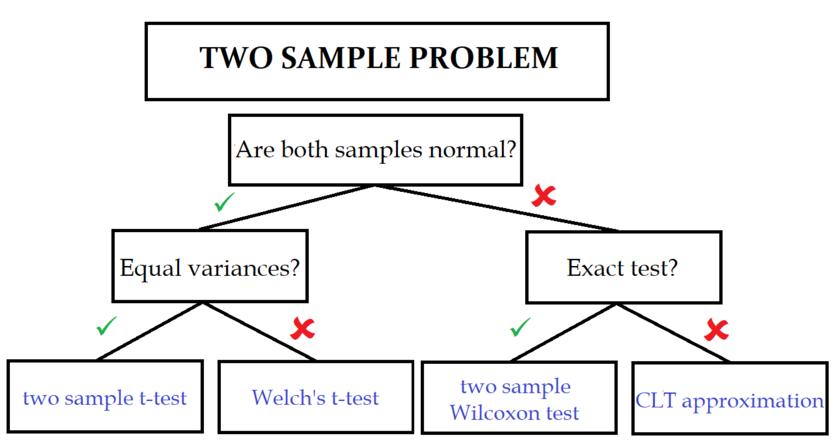
Two-sample $t$-test
The two-sample t-test (also known as the independent samples t-test) is a method used to test whether the unknown population means of two groups are equal or not.
For testing equality of means of more than two groups, we cannot repeatedly invoke two-sample $t$-test! We can use a method such as ANOVA.
- Model:
- $X_1, \dots, X_n$ is a random sample from $\mc{N}(\mu_1, \sigma^2)$
- $Y_1, \dots, Y_n$ is a random sample from $\mc{N}(\mu_2, \sigma^2)$
- both samples are mutually independent
- Null hypothesis: $H_0: \mu_1 = \mu_2$
- Test statistic: $T = \frac{\bar{X} - \bar{Y}}{S_* \sqrt{\frac{n_1 + n_2}{n_1 n_2}}}$, where $S_*$ is the pooled standard deviation
F-test
- Model:
- $X_1, \dots, X_n$ is a random sample from $\mc{N}(\mu_1, \sigma_1^2)$
- $Y_1, \dots, Y_n$ is a random sample from $\mc{N}(\mu_2, \sigma_2^2)$
- both samples are mutually independent
- Null hypothesis: $H_0: \sigma_1^2 = \sigma_2^2$ (the variances are equal)
- Test statistic: $F = \frac{S_1^2}{S_2^2}$ ($f$ has the Fisher-Snedecor F-distribution under $H_0$)
Paired $t$-test
- Model:
- $Z_1 = X_1 - Y_1, \dots, Z_n = X_n - Y_n$ is a random sample from normal distribution $\mc{N}(\mu, \sigma^2)$
- Null hypothesis: $H_0: \mu = 0$ ($X$ and $Y$ are pairwise equal)
- Test statistic: $T = \sqrt{n}\frac{\bar{Z}}{S}$
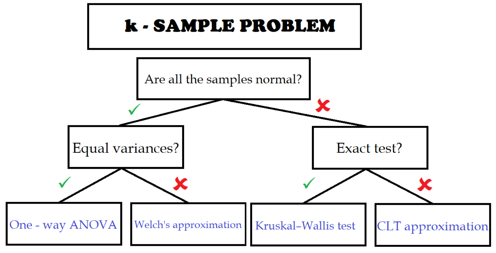
ANOVA
We want to find out whether means of $k$ groups are equal, but if we wanted to use $t$-tests for every pair, we would need to do ${k \choose 2} = c$ of the tests. For that we would need to set the confidence level of every test to $\frac{\alpha}{c}$, which makes the test procedure too conservative and the tests will have small power. ANOVA helps us to fix the problem.
- Model:
- $X_{1,1}, \dots, X_{1, n_1}$ is a random sample from $\mc{N}(\mu_1, \sigma^2)$
- $X_{2,1}, \dots, X_{2, n_2}$ is a random sample from $\mc{N}(\mu_2, \sigma^2)$
- $\vdots$
- $X_{k,1}, \dots, X_{k, n_k}$ is a random sample from $\mc{N}(\mu_k, \sigma^2)$
- all samples mutually independent, normality, same variances (homoscedasticity)
- $n = n_1 + \dots + n_k$
- Null hypothesis: $H_0: \mu_1 = \mu_2 = \dots = \mu_k$
- $H_1: \mu_i \not= \mu_j$ for at least one pair $i \not= j$.
- If $H_0$ is rejected, then we want to know which groups differ. ANOVA will not tell us that, but we can use post-hoc tests.
\[\text{SS}_T = \text{SS}_W + \text{SS}_B\]
- \(\text{SS}_T = \sum_{i = 1}^k \sum_{j = 1}^{n_i} (X_{i, j} - \bar{X})^2\) is called total sum of squares,
- \(\text{SS}_W = \sum_{i = 1}^k \sum_{j = 1}^{n_i} (X_{i, j} - \bar{X_i})^2\) is called within-group (residual) sum of squares,
- \(\text{SS}_B = \sum_{i = 1}^k n_i (\bar{X}_i - \bar{X})^2\) is called between-group sum of squares.
$\frac{\text{SS}_W}{n - k}$ is an unbiased estimate of $\sigma^2$. $\frac{\text{SS}_B}{k - 1}$ is an unbiased estimate of $\sigma^2$ only under $H_0$. The idea is to compare these two estimates using $F$-test:
- Test statistic: $F = \frac{\text{SS}_B / (k - 1)}{\text{SS}_W / (n - k)}$ (under $H_0$, $F \sim F(k - 1, n - k)$)
Post-hoc Tests
Post-hoc test is a test that is specified after the data were already analyzed by a different kind of test. For example, ANOVA made us reject the null hypothesis that the means of all the groups are the same, and now we want to know exactly which groups statistically differ.
Tukey’s HSD
Test statistic: $Q_{i, j} = \frac{\abs{\bar{X}_i - \bar{X}_j}}{S \sqrt{\frac{1}{2n_i} + \frac{1}{2n_j}}}$
- under $H_0$, follows the studentized range distribution
in one sample, two samples, more than two samples (including one sample, two sample and paired t-tests, ANOVA and post-hoc tests), goodness-of-fit tests.
Another post-hoc test used after ANOVA is for example Scheffé Test.
There is Only One Test
An interesting article to read - Monte Carlo simulation is probably enough for your hypothesis testing needs (and waaay easier to understand than these ‘arbitrarily-chosen’ super complicated test statistics).
Linear Regression Model
- One of the most popular and used statistical methods.
-
Modelling the relationship between a numerical response and one or more explanatory variables.
- Denote \(\bf{X} = \begin{pmatrix} 1 & x_{1,1} & x_{1_2} & \cdots & \cdots & x_{1, p} \\ 1 & x_{2,1} & x_{2_2} & \cdots & \cdots & x_{2, p} \\ \vdots & \vdots & \ddots & \ddots & \vdots & \vdots \\ 1 & x_{n,1} & x_{n_2} & \cdots & \cdots & x_{n, p} \\ \end{pmatrix}\) the design matrix.
- $\bf{Y} = (Y_1, \dots, Y_n)^T$ is the target/response variable (dependent variable, numerical)
-
Linear regression model:
\(Y_i = \beta_0 + \beta_1 x_{i, 1} + \beta_2 x_{i, 2} + \dots + \beta_p x_{i, p} + e_i = \bf{x}_i^T \bf{\beta} + e_i,\) $i = 1, \dots, n.$
- $\beta = (\beta_0, \beta_1, \dots, \beta_p)^T$ is the vector of unknown parameters,
- $e_i$ - (random) model error
- \(\bf{x}_i = (1, x_{i, 1}, x_{i, 2}, \dots, x_{i, p})^T\) - vector of regressors, predictors, input variables (independent variables, numerical/categorical)
Model Assumptions
- Expectation of model errors is zero (no systematic error).
- Variance of model errors is constant (homoscedasticity).
- Model errors are independent and have normal distribution.
- $e_1, \dots, e_n$ is a random sample from $\mc{N}(0, \sigma^2)$.
-
Expectation of $Y_i$ is a linear function of unknown parameters, i.e.
\[\E Y_i = \beta_0 + \beta_1 x_{i, 1} + \beta_2 x_{i, 2} + \dots + \beta_p x_{i, p}\] - Regressors are not affected by random errors.
- There are no outliers in our data.
Least Squares Estimate
- $\hat{\beta} = \arg\min\set{\sum_{i = 1}^n (Y_i - \bf{x}_i^T \bf{b})^2 : \bf{b} \in \R^{p + 1}}$
- If the rank of $\bf{X}$ is $p + 1$, then $\hat{\beta} = (\bf{X}^T \bf{X})^{-1} \bf{X}^T \bf{Y}$
- \(\hat{Y}_i = \bf{x}_i^T \hat{\beta} = \hat{\beta_0} + \hat{\beta_1}x_{i, 1} + \dots + \hat{\beta_p} x_{i, p}\).
If the rank of $\bf{X}$ is $p + 1$, then
- $\hat{\beta}$ is the best unbiased linear estimate of $\beta$,
- $\hat{\beta} \sim \mc{N}_{p + 1}(\beta, \sigma^2 (\bf{X}^T \bf{X})^{-1})$.
- $T_j = \frac{\hat{\beta_j} - \beta_j}{S \sqrt{v_{j, j}}} \sim t(n - p - 1)$, where $\bf{V} = (\bf{X}^T\bf{X})^{-1}$ has element $(v_{i, j})$
Test of Influence
- We can test whether a particular regressor has an influence on the response or not.
- Test statistic: $T_j = \frac{\hat{\beta_j}}{S \sqrt{v_{j, j}}}$
- under $H_0$, the test statistic $T_j \sim t(n - p - 1)$
- if we want to test $\beta_i = 0$ and $\beta_j = 0$ simultaneously, we cannot use this test, but test of a submodel
Test of a Submodel
- The question: Can we reduce the full model with design matrix $\bf{X}$ to submodel with design matrix $\bf{X}_0$?
- $H_0$: The submodel is true.
Coefficient of Determination
\(R^2 = 1 - \frac{\sum_{i = 1}^n (Y_i - \hat{Y_i})^2}{\sum_{i = 1}^n (Y_i - \bar{Y_i})^2}\)
Indicates the proportion of the variance in response that is explained by the model.
- $R^2$ increases when a new predictor is added to the model, even if the new predictor is not associated with the outcome.
- We can use the adjusted coefficient of determination, which penalizes for the number of predictors included in the model.
Interpretation
- $\beta_0$ is an intercept - the expected value of $Y_i$ when values of all regressors $X_i$ are equal to $0$.
- $\beta_j$ is the expected change in $Y_i$ when the value of the $j$-th regressor is changed for one unit, while other regressors are fixed.
Linear Regression - Remarks
- Disadvantages:
- Very strong assumptions.
- Sensitive to leverage observations and outliers.
- Unstable for strongly correlated regressors.
- Cannot deal with missing values.
- Works globally.
- Advantages:
- Simple interpretation.
- Direct quantification of the influence of individual regressor on the response.
- Many generalizations.
- Can deal with both numerical and categorical variables.
- Does not suffer from the curse of dimensionality.